Dynamic linkages between the US stock market and the stock markets of European economies

1. Abstract

Understanding the degree of interdependence between national stock markets and the nature of their relationship (market dominance, a transmission mechanism, and degree of responsiveness to information flows) have implications for market stability and international diversification (Eun and Shim, 1989; Chowdhury, 1994). In this paper, I will empirically examine the short-run relationships between the US stock market and the national stock markets of each of the European economies (German, Ireland, France) by investigating dynamic causal linkages between those markets using Johansen cointegration test and Vector Auto regression Estimates (VAR).

2. Literature Review

The issue of interdependence between the stock market indices is raising concern among empirical research recently. Initial researches by Granger and Morgenstem (1970), Grubel and Fadner (1971), Ripley (1973), and Lessard (1976) found small or no correlation between stock market indices from the 1960s to 1970s. Those early researches use simple methodologies such as regression and correlations.

Early studies mainly focus on the short-run relationship among national stock indices. However, Hassan and Naka (1996) studies long-run and the short-run relationships and examines multivariate linkages and lead-lag relationships among 4 daily stock market indices (U.S., Japan, U.K., and Germany) by daily data from 1984 to 1981.

Kim (2010) analyzes the dynamic causal relationship between the U.S. stock market and the East Asian stock markets at different time scales by employing wavelet analysis. Analyses of pre-crisis, East Asian financial crisis (the year 1997-2000), inter-crisis and the subprime mortgage crisis (the year 2007- 2009) periods are conducted to compare the international transmission mechanism of stock market movements.

Mustafa (2002) examine the dynamic linkages between sub-sector indices of Saudi Tadawul Stock Exchange using Johansen cointegration tests and the vector error correction model (VECM).

This research will analyze long-run and the short-run relationship of four developed country stocks (German, Ireland, France, U.S.) by using Johansen cointegration tests and VAR model to analyze the short term relationship among four stock indices

3. Data description

The data, collected from Datastream, are daily closing stock market indices for the period January 22, 2001, to March 13, 2019.  The stock market indices are France (Lyxo Cac 40), Germany (DAX), Ireland (ISEQ 20), and US (S&P 500).  Daily stock market index data are preferred because daily data can capture the speedy movement of information better than weekly, monthly or annually data, and we are finding both the short-run, long-run dynamic relationship among national stock indices. The data are quoted in US dollar and transformed to natural logarithms.

3.1. Data as natural logarithms

Table 1. Data as natural logarithms

	LnCAC	Ln S&P500	LnDAX	LnISEQ
Mean	3.940103	7.271526	4.329306	6.878232
Median	3.948305	7.185902	4.420622	6.935205
Maximum	4.459371	7.983014	4.971978	7.656555
Minimum	3.266126	6.516977	3.171365	5.892335
Std.Dev.	0.220866	0.328979	0.393416	0.350095
Skewness	-0.133367	0.448845	-0.641525	-0.047292
Kurtosis	3.062766	2.254467	2.520744	2.312149
Jarque-Bera	14.80776	268.5320	369.9441	95.07115
Probability	0.000609	0.000000	0.000000	0.000000
Sum	18648.51	34416.13	20490.61	32554.67
Sum.Sq.Dev	230.8356	512.1296	732.3990	578.9832
Observations	4733	4733	4733	4733

Table 1 presents the brief statistic of natural logarithms of daily stock indices: U.S. (S&P 500) stock and Ireland (ISEQ 20) stock are larger than France (Lyxo Cac 40), Germany (DAX). The standard deviation in time series shows that the price of France stock is more stable than price of other countries. The Jarque–Bera test is a goodness-of-fit test of whether sample data have the skewness and kurtosis matching a normal distribution. And, the result for normal distribution is significant; therefore, it can deny the null hypothesis that the data is normal distributed. In the other word, the data is not normal distributed.

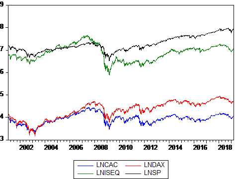
As can be seen from graph 1, four time series (natural logarithm) noticeably decrease in the same period from 2008 to 2009, which indicates a global financial crisis.There is no seasonality. There are no obvious outliers. It can be seen from the graph that the variance is not constant.

• Data at first different

First different of time series or return of stock indices will be calculated by the following equation:
Return(Yt) = log (Yt) – log (Yt-1)

Table 2. Data as first different

	ReturnCAC	ReturnDAX	Return S&P500	ReturnISEQ
Mean	0.0000139	0.000125	0.000156	0.0000631
Median	0.000485	0.000410	0.000272	0.000403
Maximum	0.113696	0.127378	0.109572	0.110390
Minimum	-0.015534	0.015644	0.011688	-0.161432
Std.Dev.	0.015534	0.015644	0.011689	0.015391
Skewness	-0.072256	-0.136415	-0.245558	-0.775077
Kurtosis	9.247754	8.414850	12.68105	12.75889
Jarque-Bera	7700.405	5795.722	18526.56	19251.13
Probability	0.000000	0.000000	0.000000	0.000000
Sum	0.065843	0.590950	0.738680	0.298809
Sum.Sq.Dev	1.141622	1.157867	0.646386	1.120707
Observations	4732	4732	4732	4732

Table 2 presents the brief statistics of daily stock return. Although from table 1, the Ireland stock index is high; however, the return of Ireland (ISEQ20) is less than half of return of U.S. (S&P 500), France (Lyxo Cac 40) and Germany (DAX). The standard deviation shows that the risk of investing in US is lower than the risk of investing in France, German and Ireland stock. The result for normal distribution is significant; therefore, the data is not normal distributed.

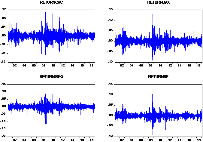
There is no clear consistent trend (upward or downward) over the entire time span.  The series wander up and down.  All of time series fluctuate around 00.0 indicates the mean of the series. 

There is no seasonality. There are no obvious outliers. It is noticeable that the first different of time series fluctuated significantly between 2008 and 2009 which indicates the huge change in finance. As can be seen from graph 2 and graph 3, there is a significant change in data in 2008 due to global financial crisis.

According to Graph 6, PACF is significant at lag order 1, and the ACF is declining very slowly, this is a common pattern indicating the presence of unit-root. Which means, lnSP is non-stationary. The ReturnSP does not exhibit strong interdependency, though lag order 1 show marginal significance.

4. Methodology

4.1. Unit root test

In order to confirm about stationary, unit root tests will be implemented. The stationary of stock indices and the first different (return) of stock indices will be tested by Agumented Dickey-Fuller(ADF) test

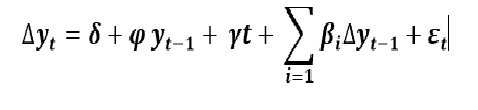
Where i= 1,2,3,..,k (k is large enough to render the white noise )

The Yt  presents the time series (or return).  ADF test regresses the first differenced series against a constant, the one period lag of the series, the differenced series at k lag lengths and a time trend. The null hypothesis for unit root test is =0  , the data is not stationary. If the time series is not stationary but the first difference of the data is stationary, it can be said that the time series is integrated at the order 1. (I(1)) [*]
* Jamil, Makwan. (2012). Short-Run and Long-Run Dynamics Linkages among the Saudi Arabia Stock Market Indices. PROSIDING PERKEM VII, JILID 2 (2012) 1624 – 1632 ISSN: 2231-962X

The ADF tests are unable to discriminate well between non-stationary and stationary series with a high degree of autocorrelation (West 1988) and are sensitive to structural breaks (Culver&Papell 1997). In addition to the DF and ADF tests, this paper will use the Phillips-Perron (PP) test (Phillips&Perron 1988), which gives the robust estimates when the series have a structural break.

Table 3. ADF and PP test

Hypothesis

H0	Unit root
H1	Stationary

Variable	ADFtc	ADFtt	PPzc	PPzt
At level
LnCAC	-2.041057	-2.294954	-2.138882	-2.405678
Ln S&P500	-0.127810	-2.565000	-0.082650	-2.488982
LnDAX	-1.228624	-2.936776	-1.173439	-2.872502
LnISEQ	-1.556919	-1.579820	-1.457967	-1.480097
5% critical value	-2.86	-3.41	-2.86	-3.41
At First difference
ReturnCAC	-33.93811***	-33.93673***	-70.36773***	-70.36287***
ReturnS&P500	-52.82578***	-52.85406***	-75.0423***	-75.09979***
ReturnDAX	-67.72308***	-67.71747***	-67.76342***	-67.75779***
ReturnISEQ	-65.83678***	-65.82993***	-65.77668***	-65.76946***
5% critical value	-2.86	-3.41	-2.86	-3.41

*ADF_tc denote that Augmented Dickey-Fuller test without trend, ADF_tt with trend, PP_(zc,zt) follows similar value as ADF’s critical value. *** Significant at 1%

As can be seen from Table 3, the results from 4 tests (ADF,PP) show that all variables in levels are non- stationary, and their difference are stationary at 5% significance level. In other words, all of time series are integrated of same order one (I(1))
4.2. Cointegration test

4.2.1. Number of lag

4.2.1.1. Vector Autoregression (VAR)

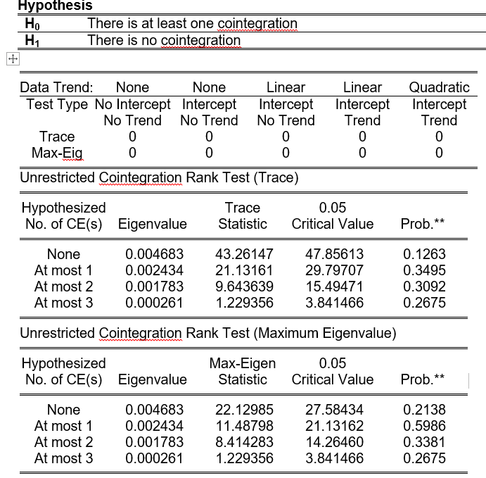
In order to choose the number of lag, Vector Autoregression Estimates (VAR) will be used. For a set of n time series variable:

For a set of n time series variables, a VAR model of order p (VAR(p)) can be written as:

where the’s are (nxn) coefficient matrices and Ut is an unobservable i.i.d. zero mean error term.  According to Chris Brooks (2014), “If one wishes to use hypothesis tests, either singly or jointly, to examine the statistical significance of the coefficients, then it is essential that all of the components in the VAR are stationary.” So VAR test will be run with the first different of data

Table 4.VAR

• 4.3. VAR Lag Order Selection Criteria

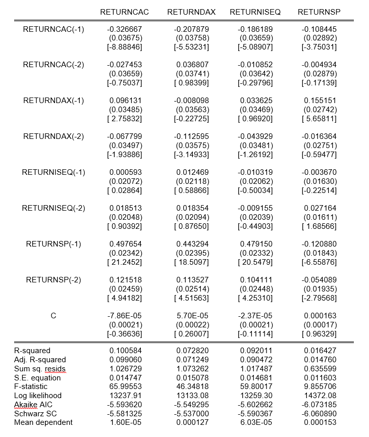
Jeffery Wooldridge’s Introductory Econometrics mentions that A Modern Approach with higher frequency data, the number of lags will be higher e.g. annual data, the number of lags is 1 or 2; for monthly data, 6, 12 lags can be used given sufficient data points. Therefore 24 lags will be chosen for daily data

Table 5. VAR Lag Order Selection Criteria

The number of lags in this test, and the subsequent tests of causality and cointegration, is determined by the Akaike Information Criterion (AIC) (Mansur M. Masih&Winduss 2006) According to usual information criteria (FPE,AIC) recommendation, lag 17 will be the optimal maximum lag length

• 4.4. Johansen test

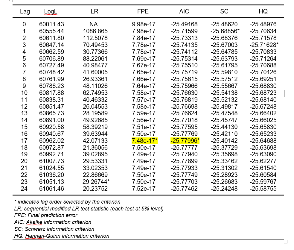
Table 6. Johansen test

As can be seen from table 6, the results are insignificant. Therefore, it can deny the null hypothesis that there is at least one cointegration; in other words, there is no cointegration among time series. So VAR model will be used to test the short-run relationship among four stock market indices.

• 4.5. VAR model and dianostics tests
  • 4.5.1. VAR model

VAR model of four Returns will be displayed as below:

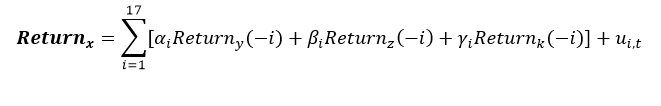
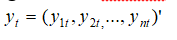
Table 7. VAR model for 17 lags

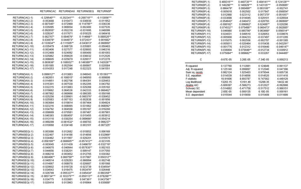
From table 7, four columns correspond to four equations in the VAR model. According to F-statistic, three model to explain four market returns has significant result means the model can explain variation of four stock markets return. The data was marked by * represent for significant result, which means the variable is affected by the past value.

• 4.5.2. Diagnostics test
  • AR Root test

The estimated VAR is stable (stationary) if all roots have modulus less than one and lie inside the unit circle. If the VAR is not stable, certain results (such as impulse response standard errors) are not valid. There will be roots, where is the number of endogenous variables and is the largest lag.

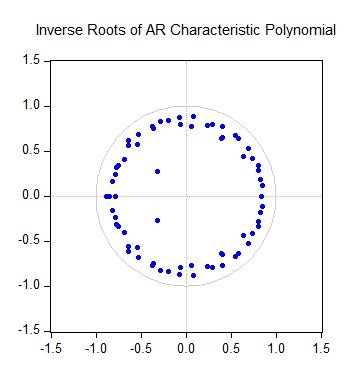
The result has shown that there is no root lies outside the unit circle; therefore, VAR satisfies the stability condition.

• Auto Correlation

In order to test the suitability of the number of lag, LM  test is taken. In this test, I will check whether lag at 17 has auto correlation.

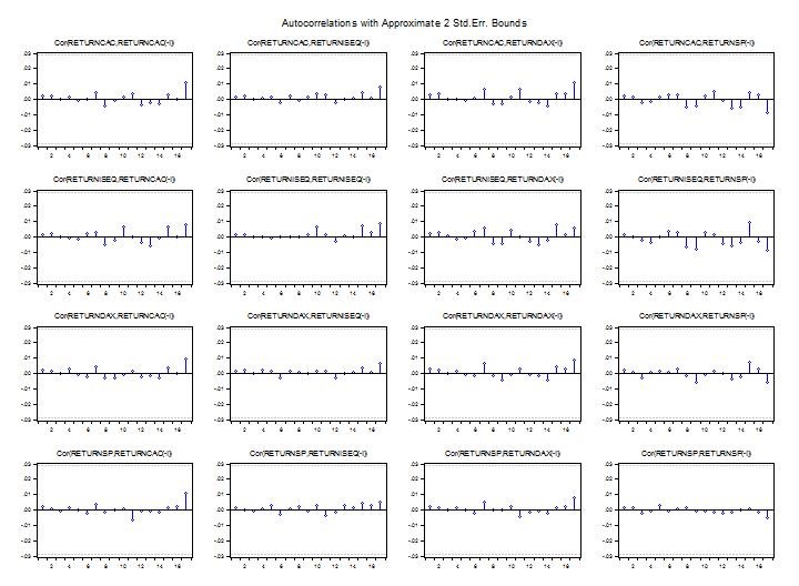
LM test has shown that the result at lag 17 is significant, so we can deny the null hypothesis.  Therefore, there is serial correlation at lag 17 and serial correlation from lag 1 to lag 17. Which indicates that one lag is sufficient for its insignificant result.

4.6. VAR Granger Causality

The Granger causality test is a statistical hypothesis test for determining whether one time series is useful in forecasting another, first proposed in 1969.[4] Multivariate Granger causality analysis is usually performed by fitting a VAR model to the time series. In particular, let  for t=1,…,T be a d-dimensional multivariate time series. Granger causality is performed by fitting a VAR model with L time lags as follows:

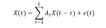
Where ɛ(t ) is a white Gaussian random vector, and  is a matrix for every, and a time series  is called a Granger cause of another time series , if at least one of the element  for  significantly larger than zero (in absolute value)[5].

Table 8. VAR Granger Causality

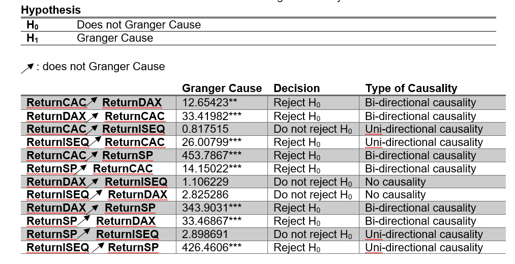
From table 8, there is Bidirectional causality exists between ReturnCAC and ReturnDAX, Uni-directional causality exists between ReturnCAC and ReturnISEQ, Bidirectional causality exists between ReturnCAC and ReturnSP, No causality exists between ReturnISEQ and ReturnDAX, Bidirectional causality exists between ReturnSP and ReturnDAX; and, Uni-directional causality exists between ReturnSP and ReturnISEQ.

4.7. Impulse response and Variance decomposition before adjusting the order

4.7.1. Impulse response

A shock to the i^th variable not only directly affects the i^th variable but is also transmitted to all of the other endogenous variables through the dynamic (lag) structure of the VAR. An impulse response function traces the effect of a one-time shock to one of the innovations on current and future values of the endogenous variables.[6]

The original order of variable: ReturnCAC, ReturnDAX, ReturnISEQ, ReturnSP

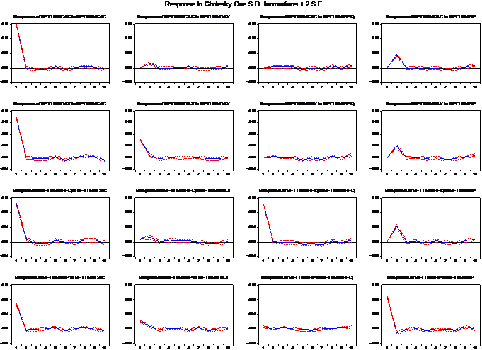
The Graph 6 has shown Impulse response without ordering, when ReturnCAC has a positive shocks, other stocks have positive reaction until 2^nd day then it has merely zero reaction. When a positive shock is given to ReturnDAX, another return has positive reaction until 3^rd day. When there is a positive shock to ReturnISEQ, other stocks nearly have no reaction except ReturnISEQ. If there is a positive shock happens to ReturnSP, other stock market returns will have positive reaction until 3^rd day, then they have negative reaction to 5^th day, after that they have no reaction. While ReturnSP has positive reaction to its own shock until day two, then it has negative reaction during day three.

• 4.7.2. Variance Decomposition

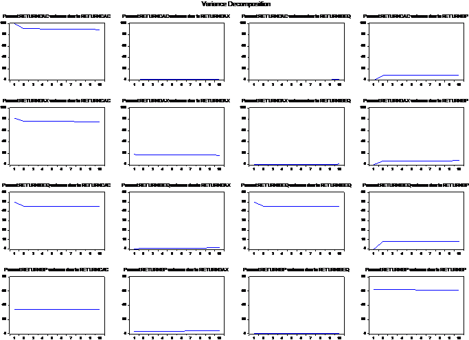
Graph 7 demonstrates that shock to ReturnCAC accounts a noticable percent for variation of the fluctuation in other returns. Impulse to ReturnSP accounts for around 7 percent for variation of the fluctuation in other returns. And, innovation to ReturnDAX accounts for around 2 percent for variation of the fluctuation in other returns. Finally, shock to ReturnSP accounts for nearly 0 percent for variation of the fluctuation in other returns.

• 4.8. Impulse Response and Variance decomposition after reorder

The U.S is a dominant economy, a shock to U.S stock exerts a substantial influence on the euro market. The German stock market has become a leading stock exchange inside the Eurozone, so the change in German stock will lead to noticeable differences in other Euro country. And if there is a shock to the French market, Ireland market stock will be influenced more than the French market will respond to a shock to Ireland market.

So we will have an order: ReturnSP, ReturnDAX, ReturnCAC, and ReturnISEQ

• 4.8.1. Impulse response after adjusting order of variables

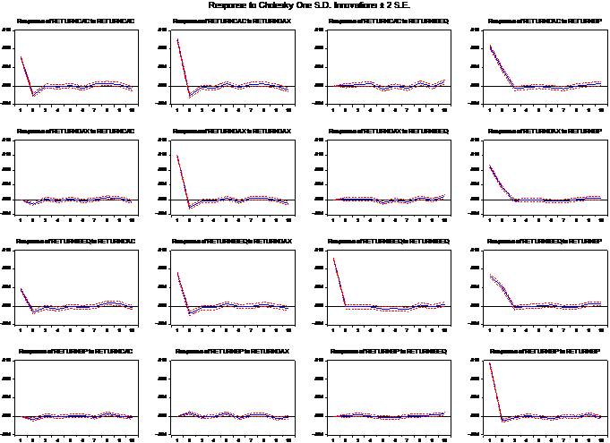
When there is a positive shock to ReturnCAC, ReturnCAC and ReturnISEQ will decrease to negative in the short run while ReturnDAX and ReturnSP has negative response in the short run. Moreover, when returnDAX has a positive shock, ReturnCAC, ReturnDAX and ReturnISEQ will greatly decrease to negative, ReturnSP will fluctuate and it has positive response innitially. Besides, if there is an appositive shock is given to ReturnISEQ, other returns of stock markets will slightly fluctuate at the beginning, and remain the same. And, when a positive shock is given to ReturnSP, three returns will has positive response and significantly decrease to negative response until day four.

• 4.8.2. Variance Decomposition

While impulse response functions trace the effects of a shock to one endogenous variable on to the other variables in the VAR, variance decomposition separates the variation in an endogenous variable into the component shocks to the VAR. Thus, the variance decomposition provides information about the relative importance of each random innovation in affecting the variables in the VAR.

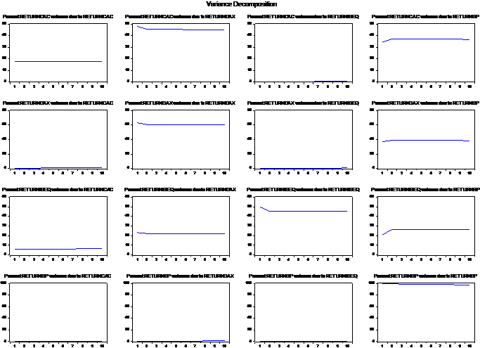
Those results show that ReturnSP accounts a significant percent for variation of the fluctuation in other returns. Impulse to ReturnISEQ accounts for less than 1 percent for variation of the fluctuation in other returns. And, innovation to ReturnDAX accounts for around 50 percent for variation of the fluctuation in other returns except ReturnSP, shock to Return DAX only accounts for around 1% of fluctuation in ReturnSP. Finally, shock to ReturnCAC accounts for less than 7 percent for variation of the fluctuation in other returns.

Comment: The results of Impulse response and Variance Decomposition after adjusting order are different from original order’s results due to Cholesky method. The adjusted results outperform the original results because the order I choose reflects my beliefs about the relationships among variables in the VAR.

5. Conclusion

This research aims to analyze the dynamic relationships among U.S., Ireland, German, France using daily data from January 22, 2001, to March 13, 2019. The short-run and long-run relationship is examined using Johansen test in this paper, which differs from early researches. On the other hand, there is no cointegration among 4 national stocks; therefore, there is no long run relationship among four stock indices and VAR model is used to examine the short-run relationship. The results is different from Hassan and Naka (1996) and Makwan(2002), in their research, there is one cointegration among daily stock market indices.

The VAR model can explain variation of four stock markets return. Several tests were taken to test the suitability of VAR model, the AR Root test shows that there is no root lies outside the unit circle; therefore, VAR satisfies the stability condition. LM test has shown that there is serial correlation at lag 17. There is Heteroskedasticity in the model, which indicates that the conclusion about significance of regression coefficients is incorrect. The Robust standard error is implemented to remove Heteroskedasticity The Residual Normality Tests have shown the significant result which indicates that the residuals are not multivariate normal.

This study finds that ReturnCAC Granger Causes ReturnDAX, ReturnDAX granger causes ReturnCAC, ReturnISEQ granger causes ReturnCAC, ReturnCAC granger causes ReturnSP, ReturnSP granger causes Return CAC, ReturnDAX granger causes ReturnSP, ReturnSP granger causes Return DAX, and ReturnISEQ granger causes ReturnSP.

Therefore, the past values of ReturnCAC, ReturnSP should contain information that helps predict ReturnDAX. Moreover,ReturnDAX, ReturnISEQ and ReturnSP is useful in predicting ReturnCAC. Besides the past values of ReturnCAC, ReturnDAX and ReturnISEQ should contain information that helps predict ReturnSP

The impulse response’s result and variance decomposition’s result is affected by ordering of variable. The results of impulse response and variance decomposition after adjusting the order of variable are better than the initial results.

According to impulse response’s result, when there is a positive shock to ReturnCAC, ReturnCAC and ReturnISEQ will decrease to negative in the short run while ReturnDAX and ReturnSP has negative response in the short run. Moreover, when returnDAX has a positive shock, ReturnCAC, ReturnDAX and ReturnISEQ will greatly decrease to negative, ReturnSP will fluctuate and it has positive response initially. Besides, if there is appositive shock is given to ReturnISEQ, other returns of stock markets will slightly fluctuate at the beginning, and remain the same. And, when a positive shock is given to ReturnSP, three returns will has positive response and significantly decrease to negative response until day four.

According to variance decomposition’s result, shock to ReturnSP accounts a significant percent for variation of the fluctuation in other returns. Impulse to ReturnISEQ accounts for less than 1 percent for variation of the fluctuation in other returns. And, innovation to ReturnDAX accounts for around 50 percent for variation of the fluctuation in other returns except ReturnSP, shock to Return DAX only accounts for around 1% of fluctuation in ReturnSP. Finally, shock to ReturnCAC accounts for less than 7 percent for variation of the fluctuation in other returns.

References

Bogl, M., Aigner, W., Filzmoser, P., Lammarsch, T., Miksch, S. and Rind, A. (2013). Visual Analytics for Model Selection in Time Series Analysis. [online] Publik.tuwien.ac.at. Available at: https://publik.tuwien.ac.at/files/PubDat_220251.pdf [Accessed 1 Apr. 2019].

Ebrary. (2019). Impulse Response and Variance Decompositions. [online] Available at: https://ebrary.net/582/economics/impulse_response_variance_decompositions [Accessed 13 Apr. 2019].

Ehrmann, M., Rigobon, R. and Fratzscher, M. (2005). Stocks, Bonds, Money Markets and Exchange Rates: Measuring International Financial Transmission. SSRN Electronic Journal.

Eviews.com. (2019). EViews Help. [online] Available at: http://www.eviews.com/help/helpintro.html#page/content%2FVAR-Views_and_Procs_of_a_VAR.html%23ww37080 [Accessed 14 Apr. 2019].

Granger, C. W. J. (1969). “Investigating Causal Relations by Econometric Models and Cross-spectral Methods”. Econometrica. 37 (3): 424–438

Hassan, M. and Naka, A. (1996). Short-run and long-run dynamic linkages among international stock markets. International Review of Economics & Finance, 5(4), pp.387-405.

Jamil, Makwan. (2012). Short-Run and Long-Run Dynamics Linkages among the Saudi Arabia Stock Market Indices. PROSIDING PERKEM VII, JILID 2 (2012) 1624 – 1632 ISSN: 2231-962X.

Kim, H. (2010). Dynamic causal linkages between the US stock market and the stock markets of the East Asian economies. The Royal Institute of technology Centre of Excellence for Science and Innovation Studies (CESIS, Paper No. 236)

Learneconometrics.com. (2019). Impulse responses and variance decompositions. [online] Available at: http://www.learneconometrics.com/class/5263/notes/gretl/Impulse%20responses%20and%20variance%20decompositions_gretl.pdf [Accessed 14 Apr. 2019].

Lütkepohl, Helmut (2005). New introduction to multiple time series analysis (3 ed.). Berlin: Springer. pp. 41–51. ISBN 978-3540262398.

Melle Hernendez, M. (2004). The Euro Effect on the Integration of the European Stock Markets. SSRN Electronic Journal.

Nber.org. (2019). Interactions of U.S. and European Financial Markets. [online] Available at: https://www.nber.org/digest/sep05/w11166.html [Accessed 16 Apr. 2019].

People.duke.edu. (2019). Identifying the orders of AR and MA terms in an ARIMA model. [online] Available at: https://people.duke.edu/~rnau/411arim3.htm [Accessed 13 Apr. 2019].

Ronayne, D. (2011). Which Impulse Response Function?. Warwick Economic Research Papers, No 971.

Wooldridge, J. (n.d.). Introductory econometrics.