Capital Asset Pricing Model (CAPM)

Various models are built to estimate mutual fund performance. However, most of these articles only deal with one, or at most two different performance models. This project will compare the most basic single factor Capital Asset Pricing Model (CAPM) as well as Fama and French model (1992,1996) add proxies for size and book-to-market; the Carhart Model (1997) introduces a stock-momentum variable[1]; and, Pastor-Stambaugh (2003) add Trade liquid variable. The project aims to compare the models and see which model is more suitable for mutual funds’ performance using STATA.

1. Mutual fund performance model

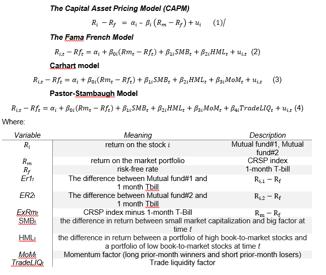
Firstly, the purpose of this project is to figure out the most suitable model for Mutual funds. Then the results will be compared to (R.Otten, D.Bams 2004)’s result: In their article, mutual funds follow the market quite closely; SMB factor loading, MoM are significantly positive, the HML factor loading on the other hand is significantly negative[2]. However, Liquid risk factor will be used in this project which isn’t examined by R.Otten, D.Bams. Therefore, two mutual funds’ performance will be compared according to coefficients of independent variables.

2. Empritical Result

2.1. Mutual fund 1

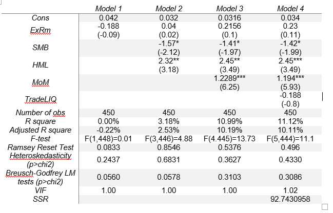
Table 1. Regression models for Mutual fund 1

2.1.1 Linear regression model test (Ramsey reset test) tests

Ramsey Reset test whether non-linear combinations of the fitted values help explain the response variable

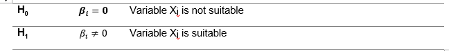
H0	the model does not have omitted-variables bias
H1	the model has omitted-variables bias

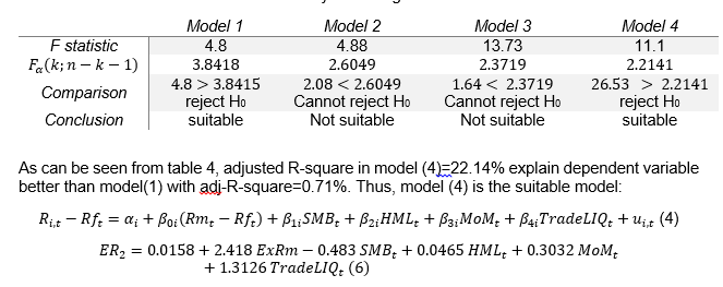
As can be seen from table 1, four modelshave Prob>F higher than 0.05, so do not reject H₀

Conclusion: four models do not have omitted-variables bias

2.1.2. Heteroskedasticity test

H0	error variances are all equal
H1	error variances are not all equal

From the test result in table 1 , the Prob>chi2 value in four model are higher than 5% indicating heteroskedasticity was probably not a problem in four models.

2.1.3. Auto Correlation test

Breusch-Godfrey LM tests

H0	ρ = 0	No Auto Correlation
H1	ρ > 0 ρ < 0	Positive Auto Correlation Negative Auto Correlation

As can be seen from table 1: Prob>chi2 in four models are higher than 0.05 => cannot reject H₀

Conclusion: There is no Auto Correlation in four models

2.1.4. Multi-collinearity test

H0	VIF< 2	Multi-collinearity doesn’t happen
H1	2<VIF<10	Multi-collinearity may happen
H2	VIF>10	Multi-collinearity sure happens

Table 2. VIF

Variable	VIF	1/VIF
MoM	1.05	0.952667
TradeLiQ	1.05	0.954738
SMB	1.01	0.992863
ExRM	1.01	0.994159
HML	1.00	0.998877
Mean VIF	1.02

As can seen from table 2 the correlation between SMB, HML, MoM , TradeLiQ, ExRM are small, so correlation doesn’t happen

Conclusion: There is no multi-collinearity

2.1.5. Test the suitability of the regression function

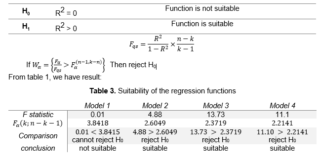
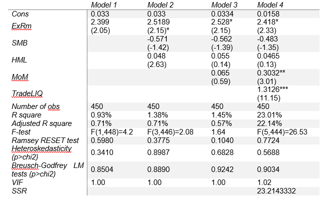
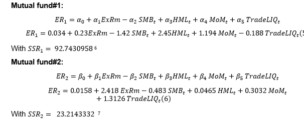
As can be seen from table 1, adjusted R-square in model(3) shows that Model(3) explains dependent variable better than model(2);and, model(3) explains slightly better than model (4). However Model(3) isn’t suitable for Mutual fund#2[5]. The purpose of project is finding suitable regression for 2 mutual funds; so, model(4) is suitable for both Mutual fund:

Model(5)’s result is different from R.Otten, D.Bams’s result: the market (ExRm) and liquid risk(TradeLIQ) has low impact on mutual fund#1; meanwhile, market capitalization(SMB) has significant and negative impact. Besides, book-to-market stocks(HML) and momentum factor(MoM) has significant and positive impact on mutualfund#1.

2.1.6. Significance of Variables

As can be seen from table 1, p-value of ExRm, TradeLIQ > 5%. Cannot reject H₀

While p- value of SMB, HML, MoM <5%.Reject H₀

Conclusion: ExRm, TradeLIQ are not statistically significant in explaining ER1.

SMB, HML, MoM are statistically significant in explaining ER1.

2.2. Mutual fund 2

Table 4. Regression models for Mutual fund 2

2.2.1. Linear regression model test (Ramsey reset test) tests

As can be seen from table 4, four modelshave Prob>F higher than 0.05 =>do not reject H₀

Conclusion: 4 models do not have omitted-variables bias

2.2.2. Heteroskedasticity test

         From the test result in table 4 , the P>chi square value in four model are higher than 5% indicating heteroskedasticity was probably not a problem in four models.

2.2.3. Auto Correlation test

As can be seen from table 4: Prob> chi square in four models are higher than 0.05 => cannot reject H₀

Conclusion: There is no Auto Correlation in four models

2.2.4.Test the suitability of the regression function

From table 4, we have result:

Table 5. Suitability of the regression functions

In from Model(6), the market (ExRm) and liquid risk (TradeLIQ) has significant and positive impact on mutual fund#2; meanwhile, market capitalization(SMB) has insignificant and negative effect. Besides, book-to-market stocks (HML) has insignificant and positive impact; and, momentum factor (MoM) has significant and positive impact on mutualfund#2.

The result is partly same as result from (R.Otten, D.Bams 2004) when mutual funds follow the market quite closely.

2.2.5. Significance of Variables

As can be seen from table 3, p-value of SMB, HML > 5%. Cannot reject H₀

While p- value of ExRm, TradeLIQ, MoM <5%.Reject H₀

Conclusion: Smb, Hml are not statistically significant in explaining ER2.

ExRm, TradeLIQ, MoM are statistically significant in explaining ER2

3. Compare two Mutual funds Performance

General regression for both mutual funds

In order to create a general regression, the new variables are created:

Create new dependent variable	Create ER by appending ER1 and ER2
Create new independent variable	Multiply all variable to create new independent variable

Table 6.General regression for both mutual funds

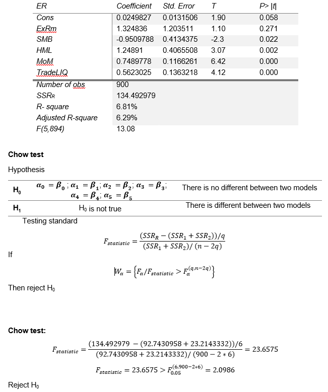
Conclusion: The relationship between two mutual funds and independent variables are different in the two Models.

Table 7: Comparison of two mutual funds’ performance

	Mutual fund1	Mutual fund 2
Cons	0.034	0.0158
ExRm	0.23 (0.11)	2.418* (2.33)
SMB	-1.42* (-1.99)	-0.483 (-1.35)
HML	2.45*** (3.49)	0.0465 (0.13)
MoM	1.194*** (5.93)	0.3032** (3.01)
TradeLIQ	-0.188 (-0.8)	1.3126*** (11.15)
Number of obs	450	450
R square	11.12%	23.01%
Adjusted R square	10.11%	22.14%
SSR	92.7430958	23.2143332

Five-factor-model can explain mutual fund 2 better than mutual fund 1 with R² _{mutual fund 2} double R² _{mutual fund 1}. However, small R² in 2 models also indicate that the model doesn’t explain both mutual funds well.

We would expect an average return of 3.4% for mutual fund#1 and 1.58% for mutual fund#2 with no market factor.

The coefficient of Market (ExRm) indicates that mutual fund 2 follows Market with beta= 2.418; meanwhile, ExRm has low impact on Mutual fund 1. Market capitalization (SMB) has negative impact on both mutual funds. However SMB has significant impact on mutual fund#1 with beta= -1.42, SMB has low effect on mutual fund#2. Book-to-market stocks (HML) and momentum factor(MoM) has positive impact on  2 mutual funds.  HML and MoM has significant impact on Mutual fund#1; meanwhile, they have low impact on Mutual fund#2. While Liquid factor has significant and positive impact on mutual fund 2 with beta = 1.3126; TradeLIQ has insignificant and negative impact on mutual fund 1.

References

D. G. Altman, J. (2018). Statistics notes: the normal distribution.. [online] PubMed Central (PMC). Available at: https://www.ncbi.nlm.nih.gov/pmc/articles/PMC2548695/ [Accessed 20 Nov. 2018].

Ghasemi, A. and Zahediasl, S. (2018). Normality Tests for Statistical Analysis: A Guide for Non-Statisticians.

Otten, R. and Bams, D. (2004). How to measure mutual fund performance: economic versus statistical relevance. Accounting and Finance, 44(2), pp.203-222.

Pastor, Lubos & Stambaugh, Robert F., 2003. “Liquidity Risk and Expected Stock Returns,” Journal of Political Economy, University of Chicago Press, vol. 111(3)

People.duke.edu. (2018). Statistical forecasting: notes on regression and time series analysis. [online] Available at: https://people.duke.edu/~rnau/411home.htm [Accessed 10 Dec. 2018]. Princeton.edu. (2018). [online] Available at: https://www.princeton.edu/~otorres/Regression101.pdf [Accessed 20 Nov. 2018].